2 Spatial statistics
2.1 Linear models for correlated errors
Motivating example
- Regression/polynomial example Download R code here
ISIT <- read.table("https://www.dropbox.com/scl/fi/n5ku9crpsr384p9z2rc8b/bioluminescence.txt?rlkey=airzs2ukql4g0hqxjr72re53j&dl=1",
    header = TRUE)

Sources16 <- ISIT$Sources[ISIT$Station == 16]
Depth16 <- ISIT$SampleDepth[ISIT$Station == 16]
Sources16 <- Sources16[order(Depth16)]
Depth16 <- sort(Depth16)
plot(Depth16, Sources16, las = 1, ylim = c(0, 65), col = rgb(0, 0, 0, 0.25), pch = 19,
    ylab = "Density of bioluminescence", xlab = "Depth in meters")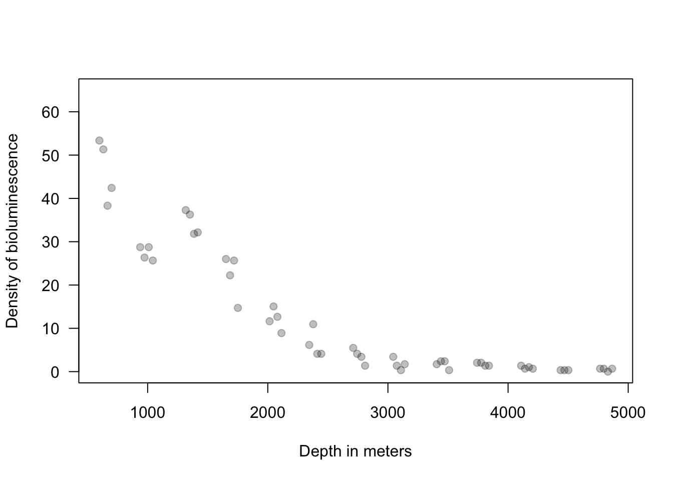
Linear model with correlated errors (aka Kriging)
- \(\mathbf{\textbf{y}}=\mathbf{X}\boldsymbol{\beta}+\boldsymbol{\eta}+\boldsymbol{\varepsilon}\) where \(\boldsymbol{\eta}\sim\text{N}(\mathbf{0},\sigma_{\eta}^{2}\mathbf{R}(\phi))\) and \(\boldsymbol{\varepsilon}\sim\text{N}(\mathbf{0},\sigma_{\varepsilon}^{2}\mathbf{I})\)
- The model above is the same as \(\mathbf{y}\sim\text{N}(\mathbf{X}\boldsymbol{\beta},\sigma_{\eta}^{2}\mathbf{R}(\phi)+\sigma^{2}\mathbf{I})\)
- Estimation
- Regression coefficients \[\hat{\boldsymbol{\beta}}=(\mathbf{X}^{\prime}\mathbf{V}^{-1}\mathbf{X})^{-1}\mathbf{X}^{\prime}\mathbf{V}^{-1}\mathbf{y}\] where \(\mathbf{V=}\sigma_{\eta}^{2}\mathbf{R}(\phi)+\sigma_{\varepsilon}^{2}\mathbf{I}\)
- Numerical maximization to estimate \(\sigma_{\eta}^{2}\), \(\sigma^{2}\), and \(\phi\)
- Error terms \[\hat{\boldsymbol{\eta}}=\hat{\sigma}_{\eta}^{2}\mathbf{R}(\hat{\phi})(\hat{\sigma}_{\varepsilon}^{2}\mathbf{I}+\hat{\sigma}_{\eta}^{2}\mathbf{R}(\hat{\phi}))^{-1}(\mathbf{y}-\mathbf{X}\hat{\boldsymbol{\beta}})\] \[\hat{\boldsymbol{\varepsilon}} = \mathbf{y} - \mathbf{X}\hat{\boldsymbol{\beta}} - \hat{\boldsymbol{\eta}}\]
Bioluminescence example
- Intercept only linear model
ISIT <- read.table("https://www.dropbox.com/scl/fi/n5ku9crpsr384p9z2rc8b/bioluminescence.txt?rlkey=airzs2ukql4g0hqxjr72re53j&dl=1",
    header = TRUE)

Sources16 <- ISIT$Sources[ISIT$Station == 16]
Depth16 <- ISIT$SampleDepth[ISIT$Station == 16]
Sources16 <- Sources16[order(Depth16)]
Depth16 <- sort(Depth16)

m1 <- lm(Sources16 ~ 1)
e.hat.m1 <- residuals(m1)

plot(Depth16, e.hat.m1, xlab = "Depth (m)", ylab = expression(hat(epsilon)), ylim = c(-15,
    60), las = 1, col = rgb(0, 0, 0, 0.25))
abline(a = 0, b = 0)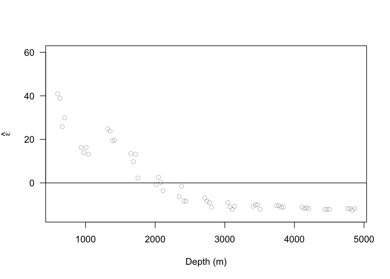
- Intercept only linear model with spatial random effect
library(nlme)
m2 <- gls(Sources16 ~ 1, correlation = corGaus(form = ~Depth16, nugget = TRUE, value = c(100,
    0.05), fixed = FALSE), method = "ML")

summary(m2)
## Generalized least squares fit by maximum likelihood ## Model: Sources16 ~ 1 ## Data: NULL ## AIC BIC logLik ## 296.3003 304.0276 -144.1502 ## ## Correlation Structure: Gaussian spatial correlation ## Formula: ~Depth16 ## Parameter estimate(s): ## range nugget ## 610.73574379 0.01300607 ## ## Coefficients: ## Value Std.Error t-value p-value ## (Intercept) 17.73824 8.981483 1.974978 0.0538 ## ## Standardized residuals: ## Min Q1 Med Q3 Max ## -0.8937320 -0.8247052 -0.6866517 0.3991341 1.7952883 ## ## Residual standard error: 19.84738 ## Degrees of freedom: 51 total; 50 residual# estimated range & nugget parameters from gls phi <- exp(m2$model[1]$corStruct[1])^2 nugget <- 1/(1 + exp(-m2$model[1]$corStruct[2])) X <- rep(1, length(Sources16)) y <- Sources16 sigma2.eta <- (m2$sigma^2) * (1 - nugget) R <- exp(-as.matrix(dist(Depth16, diag = TRUE, upper = TRUE))^2/phi) sigma2.e <- (m2$sigma^2) * nugget I <- diag(1, length(y)) V <- sigma2.eta * R + sigma2.e * I beta <- solve(t(X) %*% solve(V) %*% X) %*% t(X) %*% solve(V) %*% y eta <- sigma2.eta * R %*% solve(V) %*% (y - X %*% beta) par(mar = c(5.1, 4.1, 2.1, 2.1), oma = c(0, 0, 0, 0)) # reset plot margins par(mfrow = c(1, 2)) # plot layout par(pch = 19) # plotting symbol # plot predictions for second-order spatial model plot(Depth16, Sources16, xlab = "Depth (m)", ylab = "Density of bioluminescence", ylim = c(-15, 60), las = 1, col = rgb(0, 0, 0, 0.25)) lines(Depth16, X %*% beta + eta, col = "black") lines(Depth16, X %*% beta, col = "purple") e.hat.m2 <- y - (X %*% beta + eta) plot(Depth16, e.hat.m2, xlab = "Depth (m)", ylab = expression(hat(epsilon)), las = 1, col = rgb(0, 0, 0, 0.25))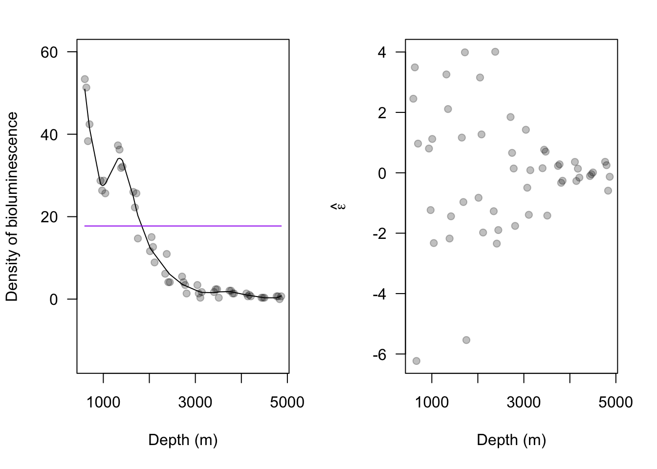
2.2 Parking lot example
- Download R code here